Multi-view learning with Deep Architectures (Generative Models)

In the previous post, we have seen Multi-view learning approaches concentrated on CCA based methods. In this article, we discuss the deep architectures used to learn from multi-view data. With the success of deep neural networks there are different approaches proposed to capture correlations between multiple views of the data. We divide these approaches from the perspective of generative versus direct common space representation learning methods. In this article, we concentrate on generative models.

Deep Multi-View Generative Models

Goal of generative models is to train on huge amount of data to generate it back. There are several studies [1] conducted earlier to understand the effectiveness of generative against discriminative models. A generative model learns the joint probability distribution $P(\mathcal{X},\mathcal{Y})$ between observed data $\mathcal{X}$ and their labels $\mathcal{Y}$ . It is then estimated using maximum likelihood (MLE) or maximum a posteriori (MAP). Main advantage of the generative models is to attribute missing data and also generate unseen data.

There are several well known generative models exist such as hidden markov models (HMM) [2], latent Dirichlet allocation (LDA) [3], restricted boltzmann machines (RBM) [4] and variational autoencoders [5.1]. In the following, we focus on models that were leveraged to learn from multiple views of the data.

Multi-View Deep Boltzmann Machines

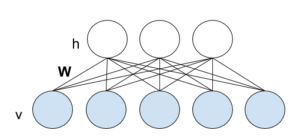
The deep Boltzmann machines (DBM) [5.2] are extension of RBM with more than one hidden layer. A binary-valued input data RBM is a undirected bipartite graphical model consisting of stochastic visible $v \in \{0,1\}^{\mathcal{R}^v}$ and 1-layer of hidden $h \in \{0,1\}^{\mathcal{R}^h}$ units which can be visualized in Figure-1.

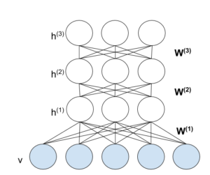
**Figure-1:** RBM with one visible (v) and hidden (h) layer along with connection weights (W)

Extending this RBM with more hidden layers enable deep learning. But connections are only allowed between adjacent hidden layers. Figure-2 shows a example DBM with three hidden layers and one visible layer.

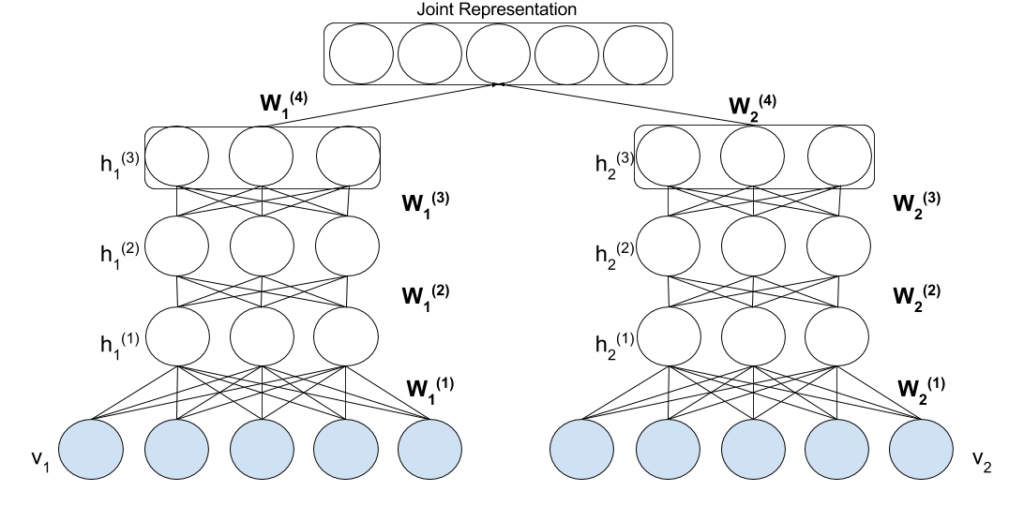
**Figure-2:** DBM with one visible layer (v) and multiple hidden layers (h*) with connection weights (W*)

Extending the architecture of DBM to the multi-view scenario involve usage of two separate DBM for each view along with an additional hidden layer to learn the joint representation. Let $v_1 \in \mathcal{R}^{v_1}$ and $h_1 \in \mathcal{R}^{h_1}$ represent visible and hidden units respectively of view-1, while $v_2 \in \mathcal{R}^{v_2}$ and $h_2 \in \mathcal{R}^{h_2}$ represent visible and hidden units respectively of view-2. Figure-3 shows the sample architecture of the multi-view DBM.

**Figure-3:** Multi-View Deep Boltzmann Machine

Now modeling the joint distribution over these multiple input views is given by

$P(v_1,v_2 ; \theta) = \sum\limits_{h^{(3)}_1,h^{(3)}_2,h^{(4)}} P(h^{(3)}_1,h^{(3)}_2,h^{(4)})(\sum\limits_{h^{(1)}_1,h^{(2)}_1,h^{(3)}_1} P(v_1,h^{(1)}_1,h^{(2)}_1,h^{(3)}_1)) (\sum\limits_{h^{(1)}_2,h^{(2)}_2,h^{(3)}_2}P(v_2,h^{(1)}_2,h^{(2)}_2,h^{(3)}_2))$

where $P(v_1,h^{(1)}_1,h^{(2)}_1,h^{(3)}_1)$ and $P(v_2,h^{(1)}_2,h^{(2)}_2,h^{(3)}_2)$ represent the joint distribution of visible and hidden units for view-1 and view-2 respectively provided by:

$P(v_1,h^{(1)}_1,h^{(2)}_1,h^{(3)}_1; \theta ) = \frac{1}{\mathcal{Z(\theta)}}exp(-E(v_1,h^{(1)}_1,h^{(2)}_1,h^{(3)}_1;\theta))$

$P(v_2,h^{(1)}_2,h^{(2)}_2,h^{(3)}_2; \theta ) = \frac{1}{\mathcal{Z(\theta)}}exp(-E(v_2,h^{(1)}_2,h^{(2)}_2,h^{(3)}_2;\theta))$

where $E(v,h^{*})$ represent the energy function provided by

$E(v_1,h^{(1)}_1,h^{(2)}_1,h^{(3)}_1;\theta) = -v^{T}_1W^{(1)}_1h^{(1)}_1-h^{(1)}_1W^{(2)}_1h^{(2)}_1-h^{(2)}_1W^{(3)}_1h^{(3)}_1$

$E(v_2,h^{(1)}_2,h^{(2)}_2,h^{(3)}_2;\theta) = -v^{T}_2W^{(1)}_2h^{(1)}_2-h^{(1)}_2W^{(2)}_2h^{(2)}_2-h^{(2)}_2W^{(3)}_2h^{(3)}_2$

To learn model parameters, approximation learning techniques such as mean-field inference [6] to estimate data dependent expectations is used, while markov chain monte carlo (MCMC) based stochastic approximation [7] are adopted to approximate model expected statistics as exact MLE learning is intractable.

Multi-View Generative Adversarial Networks

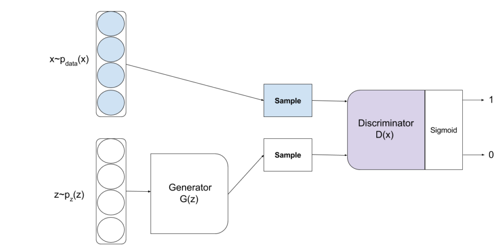
The generative adversarial networks (GANs) [8] are an approach to make two neural networks compete with each other. A generator neural network emulate the random noise into true distribution of the data in an attempt to fool the discriminator neural network whose goal is to distinguish genuine data from the imitation data created by the generator network. There are several variations [9] of GANs exist. But in the following, we explore a GAN which leverages multi-view data. A Multi-view GAN is expected to perform density estimation from multi-view inputs and also can deal with missing views to update its prediction when more views are provided.

First, we illustrate the concept of GAN. Given an input data $x$ , prior $p_z(z)$ over input noise variables is defined along with a differentiable generative function $G(z;\theta_g)$ and discriminator $D(x;\theta_d)$ function over input data $x$ to predict a single scalar. $D$ and $G$ are now trained to maximize and minimize the label prediction and $log(1-D(G(z)))$ respectively with two-player minimax game [10] using a value function $V(G, D)$ provided by:

$\min\limits_{G} \max\limits_{D} V(D,G) =\mathop{\mathbb{E}}_{x \sim p_{data}(x)}[log(D(x)]+\mathop{\mathbb{E}}_{z \sim p_{z}(z)}[log(1-D(G(z))]$

Figure-4 visualize the entire process.

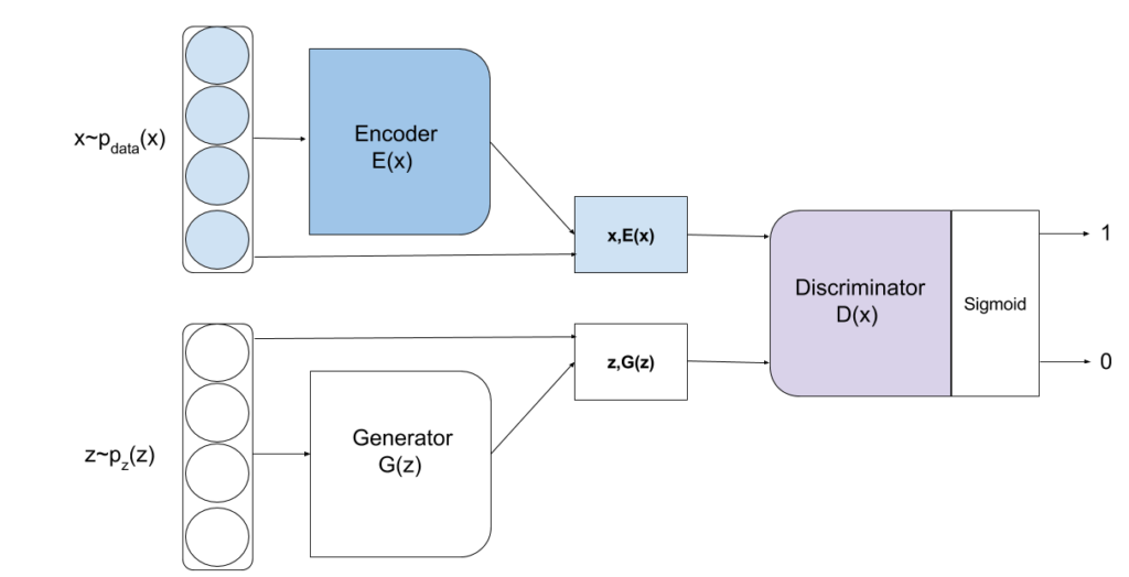
**Figure-4:** Generative Adversarial Network (GAN)

However, modeling multi-view GANs still require more sophistication than the basic GAN provides. Thus, Bidirectional GANs (BiGANs) [11] are leveraged as they can learn inverse mapping between feature representations and the input noise variables. This helps to get back the learned latent feature representations useful for many auxiliary tasks .

The BiGAN introduces additional encoder $E (x)$ which induces distribution $p_E(z|x)$ along with generator $G$ that models distribution $p_G(x|z)$ . Discriminator $D$ is modified now to take input from both $x,z$ and aim to comprehend whether the sample is generated from $p_E(z|x)$ or $p_G(x|z)$ . Thus the modified training objective is provided by:

$\min\limits_{G,E} \max\limits_{D} V(D,E,G) =\mathop{\mathbb{E}}_{x \sim p_{data}(x)}[\mathop{\mathbb{E}}_{z \sim p_{E}(.|x)}[log(D(x,z)]]+\mathop{\mathbb{E}}_{z \sim p_{z}(z)}[\mathop{\mathbb{E}}_{z \sim p_{G}(.|z)}[log(1-D(x,z)]]$

Figure-5 visualizes the BiGAN process.

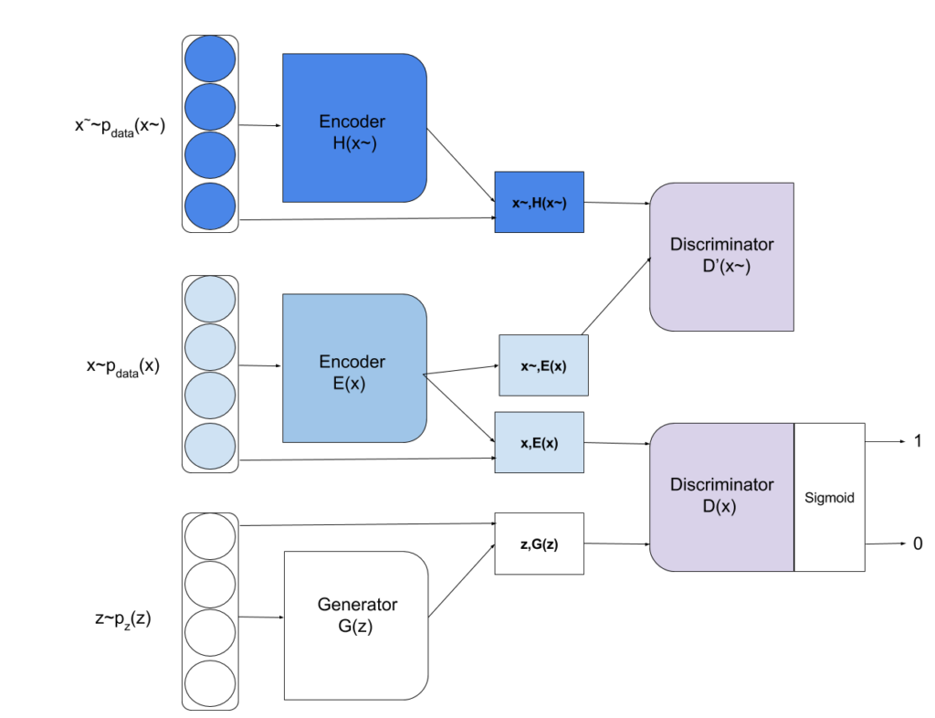
**Figure-5:** Bidirectional GAN with Encoder, Generator and Discriminator.

The BiGANs are further modified into Multi-view BiGAN [12] to support the learning from multiple views of data. The model is built on the principle that adding one more view to any subset of views must decrease the uncertainty on the output distribution. Multi-view introduces new encoder function $H$ to leverage multiple views represented with $\widetilde{x}$ to model distribution $p_{H}(z|\widetilde{x})$ and also a discriminator $D'$ such that the divergence between the $P_{E}(z|x)$ and $P_{H}(z|\widetilde{x})$ can be calculated $V(E,H,D')$ as provided by:

$\min\limits_{E,H} \max\limits_{D'} V(E,H,D') =\mathop{\mathbb{E}}_{\widetilde{x} \sim p_{data}(\widetilde{x})}[\mathop{\mathbb{E}}_{z \sim p_{E}(z|x)}[log(D'(x,z)]]+\mathop{\mathbb{E}}_{\widetilde{x} \sim p_{data}(\widetilde{x})}[\mathop{\mathbb{E}}_{z \sim p_{H}(z|x)}[1-log(D'(\widetilde{x},z)]]$

Combining the objective of BiGANs i.e. V(D,G,E) with V(E,H,D’) provide the final objective of single-view BiGAN and easily extended to $N$ different views (assuming all views are available) with the aggregation model provided by:

$\Psi(\widetilde{x}_k) = \sum\limits_{k=1}^N \Phi (\widetilde{x}_k)$

where $\Phi (\widetilde{x}_k)$ represent the usage of different views from $\widetilde{x}$ . Figure-6 visualizes the Multi-View BiGANs process.

**Figure-6:** Multi-View GAN with two encoders, generator and two discriminators

If neural networks architectures are used for generator and discriminator. Then to learn model parameters, mini-batch stochastic gradient can used.

Applications

Multi-View generative models is been applied to many applications. Mainly it is used to learn from multiple views provided by different modalities using a Multimodal DBM [13] to generate one modality from another. It has also been employed for joint representation of questions and answers for predicting answers to unseen questions [14]. Deep multimodal DBM was also explored for emotion prediction in videos [15] and is exploited for fusing visual, auditory, and textual features.

Multi-View GANs has been applied to generate faces [16] from different views.

References

[1] Ng, A.Y. and Jordan, M.I. On discriminative vs. generative classifiers: A comparison of logistic regression and naive bayes. In NIPS (2002).

[2] Blunsom, P. Hidden markov models. Lecture notes. (2004)

[3] Blei, D.M., Ng, A.Y. and Jordan, M.I. Latent dirichlet allocation. Journal of machine Learning research. (2003)

[4] Hinton, G. A practical guide to training restricted Boltzmann machines. Momentum. (2010)

[5.1] Kingma, D.P. and Welling, M. Auto-encoding variational bayes. arXiv preprint arXiv:1312.6114. (2013)

[5.2] Salakhutdinov, R. and Hinton, G. Deep boltzmann machines. In Artificial Intelligence and Statistics.(2009)

[6] Xing, E.P., Jordan, M.I. and Russell, S. A generalized mean field algorithm for variational inference in exponential families. In Proceedings of the Nineteenth conference on Uncertainty in Artificial Intelligence. (2002)

[7] Andrieu, C., De Freitas, N., Doucet, A. and Jordan, M.I. An introduction to MCMC for machine learning. Machine learning. (2003)

[8] Goodfellow, I., Pouget-Abadie, J., Mirza, M., Xu, B., Warde-Farley, D., Ozair, S., Courville, A. and Bengio, Y., 2014. Generative adversarial nets. In Advances in neural information processing systems. (2014)

[9] https://github.com/hindupuravinash/the-gan-zoo

[10] Truscott, T.R. Techniques used in minimax game-playing programs (Doctoral dissertation, Duke University).(1981)

[11] Donahue, J., Krähenbühl, P. and Darrell, T. Adversarial feature learning. arXiv preprint arXiv:1605.09782. (2016)

[12] Chen, M. and Denoyer, L. Multi-view Generative Adversarial Networks. arXiv preprint arXiv:1611.02019. (2016)

[13] Srivastava, N. and Salakhutdinov, R.R. Multimodal learning with deep boltzmann machines. In Advances in neural information processing systems. (2012)

[14] Hu, H., Liu, B., Wang, B., Liu, M. and Wang, X. Multimodal DBN for Predicting High-Quality Answers in cQA portals. In ACL. (2013)

[15] Pang, L. and Ngo, C.W. Mutlimodal learning with deep boltzmann machine for emotion prediction in user generated videos. In Proceedings of the 5th ACM on International Conference on Multimedia Retrieval. (2015)

[16] Liu, Z., Luo, P., Wang, X. and Tang, X. Deep learning face attributes in the wild. In Proceedings of the IEEE International Conference on Computer Vision (2015).