LLM Inference – Chapter-3 – Fast and Cheap for Agentic AI

In the previous chapters (chapter-1 and chapter-2), we have looked into the hardware and the software stacks that help to host Large Langue Models (LLM) and support their inference. In this chapter, we look into the Agentic workflows that are driven by LLM inference and the approaches that are designed to make the LLM inference faster and cheaper.

AI agents are becoming central to enterprise automation, but their multi-step, multi-call nature creates compounding costs and latency. A single user query can trigger dozens of LLM calls, tool invocations, and retry chains. Without deliberate optimization, inference bills scale unpredictably and response times degrade.

This chapter focuses on the key strategies for building agents that are both faster and cheaper. The core insight is that optimization is not a single technique but a layered stack: choosing the right model size by leveraging small language models (SLMs), caching repeated context, minimizing token waste, batching requests efficiently, routing to appropriate models, and engineering for tail latency. Teams that stack these techniques report 60–90% cost reductions and order-of-magnitude latency improvements.

Why We Need Cheaper Inference for Agentic AI

Let’s understand this for an unoptimized agent which is required to process Tk messages daily and is dependent on frontier models like Gemini 3.1 Pro or Claude Opus 4.6. Let’s assume that its models process Tk input tokens. The following simulation shows the cost per month.

Model Pricing (example: June 2026)

Model	Input (per 1M tokens)	Output (per 1M tokens)
Gemini 3.1 Pro	$2.00	$12.00
Claude Opus 4.6	$5.00	$25.00

Since it is an unoptimized agent, no prompt caching, no batch API, no optimization is applied.

Cost Simulation Table

The table below shows estimated monthly costs by varying daily input token volume.

Daily Input (Tk)	Monthly Input Tokens	Monthly Output Tokens	Gemini 3.1 Pro	Claude Opus 4.6
100k	3M	600k	$13.20	$30.00
500k	15M	3M	$66.00	$150.00
1M	30M	6M	$132.00	$300.00
5M	150M	30M	$660.00	$1,500
10M	300M	60M	$1,320	$3,000
50M	2B	300M	$6,600	$15,000
100M	3B	600M	$13,200	$30,000
500M	15B	3B	$66,000	$150,000
1B	30B	6B	$132,000	$300,000

Monthly Cost = (Daily_Input × 30 days × Input_Price/1M) + (Daily_Input × 0.20 × 30 days × Output_Price/1M)

To understand the expenses: At 10M tokens/day (a modest production agent handling ~5k–10k messages), costs reach $1.3k–$3k/month. At 100M+ tokens/day (high-volume enterprise agent), costs hit $13k–$30k/month without optimization.

Building An Optimized Agent

As discussed, building an optimized agent requires a combination of different techniques including leveraging caching, SLMs, batching and so on. We understand what are the approaches typically used to achieve it.

Small Language Models (SLMs): The Right Default for Agents

The Core Thesis

NVIDIA researchers (Belcak et al., arXiv 2506.02153) argue that small language models (SLMs, typically 1–10B parameters) are “sufficiently powerful, inherently more suitable, and necessarily more economical for many invocations in agentic systems.” The key observation is that inside an agent loop, the language model performs a small number of specialized tasks repetitively with little variation—routing inputs, extracting fields, deciding which tool to call, and formatting results.

Why SLMs Win for Agent Workloads

Cost efficiency: Serving a 7B SLM is 10–30x cheaper (in latency, energy, and FLOPs) than a 70–175B LLM.
Speed: On-device SLMs serve tokens in tens of milliseconds versus hundreds of milliseconds for cloud frontier LLMs.
Behavioral alignment: SLMs fine-tuned for specific output formats (JSON, tool calls) produce more predictable, schema-compliant outputs with fewer hallucinations.
Fine-tuning agility: Parameter-efficient fine-tuning (LoRA, DoRA) requires only a few GPU-hours, enabling overnight iteration.

Key Benchmarks

Phi-4-mini (3.8B): Matches Llama 3.1 8B on MMLU (73%) at half the memory
Qwen3-4B: Scores 83.7 on MMLU-Redux, beating models up to twice its size
xLAM-2-8B (Salesforce): Surpasses GPT-4o and Claude 3.5 on tool calling
DeepSeek-R1-Distill-Qwen-7B: Outperforms Claude-3.5-Sonnet on reasoning
Berkeley Function Calling Leaderboard: 1–3B models handle reliable single-turn tool use; 7–20B with fine-tuning match GPT-4-class tool use

The SLM-First Hybrid Pattern

The recommended architecture is SLM-first with cloud escalation. The agent runs a local small model on every step. A lightweight router watches for low confidence or schema violations and escalates only those turns to a frontier cloud model. Practitioners report this keeps 80–90% of agentic steps in the cheap local lane. The result is a system where 40–70% of tasks previously handled by LLMs can be offloaded to SLMs (Omdena).

On-Device Deployment and SLM-First Architectures

The On-Device Lineup

Modern quantization techniques make capable agents fit in minimal memory:

Phi-4-mini (3.8B): ~3 GB at Q4, 128K context, MIT license
Gemma 3 1B: 0.5 GB at int4 QAT, smartphone-class
Gemma 3 4B: 2.6 GB at int4 QAT, runs on 4 GB GPU / 8 GB Mac
Gemma 4 E2B: <1 GB in LiteRT-LM mobile format
Qwen3 1.7B: ~1.1 GB, strong native tool calling
Nemotron Nano 4B: ~3 GB, RL-trained for tool calling
Apple Foundation Model (~3B): On-chip Neural Engine, Swift @Generable API

Tool Calling at Small Scale

The Berkeley Function Calling Leaderboard shows that 1–3B is the sweet spot for reliable single-turn tool use on edge devices. Models below 1B fail reliably on multi-turn, parallel-function, and nested calls. Above the band, 7–20B models with fine-tuning can match or beat closed proprietary systems. The practical implication: map each agentic step to the lane it belongs in—mechanical work the SLM owns, and genuinely hard turns you escalate.

Break-Even Economics

At an illustrative rate of $1.00/M input tokens and $5.00/M output tokens with ~2,000 tokens per step (~$0.004/step):

1,000 steps/day: $4/day cloud cost → $600 machine pays for itself in 150 days
5,000 steps/day: $20/day → break-even in 30 days
10,000 steps/day: $40/day → break-even in 15 days
50,000 steps/day: $200/day → break-even in 3 days

With SLM-first routing keeping 80–90% of steps local, actual cloud spend is only 10–20% of the cloud-only cost. For many teams, the “hardware” is a laptop they already own, making break-even immediate.

Privacy and Compliance Advantage

On-device inference means no user data is transmitted externally. For GDPR, HIPAA, and data-residency regimes, this is a native compliance advantage: no cross-border transfer, no third-party processor in the inference path. Only escalated turns reach the cloud, and per-task rules can prevent sensitive content from escalating at all.

KV Caching and Prefix Caching

The Problem: Agents Pay to Re-Read Every Turn

Every agent builder knows the pattern: a long system prompt, tool catalog, few-shot examples, growing conversation history, and a ReAct loop. Each time the agent calls the model, it resends most of that context. The model quietly redoes the same compute. For an agent performing dozens of LLM calls in a single task, this adds up to massive wasted spend.

How KV Caching Works

When a transformer processes a prompt, it computes Key and Value vectors at every layer for each token. These KV tensors encode the model’s understanding of the prompt. Computing them is the “prefill” phase—and for long prompts, prefill dominates both latency and cost. Once computed, generating each new output token is comparatively cheap.

If the model keeps the KV cache between calls or shares it across requests, the agent gets faster and cheaper without changing a line of code. Most of an agent’s bill is the prefill phase, and most of the prefill is recomputing context the model has already seen.

Why Agents Pay the Highest “Inference Tax”

Heavy stable prefix: System prompt and tool catalog are identical for the agent’s lifetime
High call volume per task: A single user request triggers dozens of LLM calls, each re-paying for the prefix
Long growing trajectories: ReAct and multi-agent patterns accumulate context—every step re-reads everything before it
Cross-session reuse: Thousands of conversations/day all start with the same setup

Implementation Approaches

Self-hosted (vLLM): Enable with --enable-prefix-caching flag. Tune --block-size and --kv-cache-memory-bytes for your workload. SGLang with RadixAttention and LMCache are alternatives.

API Providers:

OpenAI: Automatic caching for prompts >1,024 tokens; cached input up to 90% off base price. Structure prompts with static parts first.
Anthropic: Enable with cache-control parameter; cached inputs 90% off but 2x cost to store. TTL ~5–10 min, extendable to 1 hour.
Tensormesh: $0 on cached input tokens as a permanent pricing feature. Exposes KV cache as a programmable surface with CPU offloading and external storage persistence.

Tensormesh Inference Platform

Tensormesh is purpose-built for this problem. Key capabilities:

KV cache CPU offloading: Push prefixes not actively in use to cheaper host memory
KV cache external storage: Persist caches to object/block storage so they survive restarts and autoscaling
Observability: See which prefixes are cached, where they live, and hit rates
Elasticity: Scale inference fleet without losing warm caches
Up to 10x reductions in latency and GPU spend reported

Typical Savings from Caching

Long system prompt apps: 50–70% on input cost
RAG with reused chunks: 40–80% depending on chunk reuse rate
Agent traces with stable instructions: up to 90% on the static prefix
Prompt caching + semantic caching combined: can reduce monthly cost from ~$1,000 to ~$50–100

Token Optimization Strategies

Strategy 1: Prompt Caching (Reuse Tokens)

The quickest win. Structure prompts with stable instructions, examples, and tool definitions first, variable content later. For API providers, this triggers automatic prefix caching that reduces input token costs by up to 90%. For self-hosted inference, enable prefix caching in vLLM or use LMCache.

Strategy 2: Semantic Caching

Match requests by meaning using embeddings and cosine similarity. If a similar enough request has been seen before, return the cached result without calling the LLM. Redis reports up to 68.8% fewer API calls and 40–50% latency improvement for Q&A workloads. Trade-offs include threshold tuning, TTL management, multi-turn complications, and risk of returning stale answers. Best suited for generic Q&A bots with high repetition.

Strategy 3: Lazy-Loading Tools and Context

Don’t preload all tool definitions into the prompt. Anthropic’s Advanced Tool Search feature keeps the always-loaded context slim and fetches tool schemas on demand via BM25 or regex search. This reduces prompt bloat from 55K–134K tokens to a fraction, while improving tool selection accuracy. The pattern: keep a compact index always loaded, fetch details only when needed.

Strategy 4: Model Routing and Cascading

60%+ of incoming queries are “easy” tasks that don’t need a frontier model. Route simple requests to cheap models, escalate complex ones. Approaches:

Predictive routing: RouteLLM (LMSYS), keyword/heuristic routing, embedding nearest-neighbor
Cascading: Let the cheap model try first; if confidence is low (logprobs, entropy), escalate
Subagents: Delegate specific tasks to smaller models (e.g., Claude Code’s Explore subagent uses Haiku)

CascadeFlow claims 69% savings and 96% quality retention vs GPT-5. Smart routing delivers 30–70% blended cost reduction on mixed-difficulty traffic.

Strategy 5: Context Hygiene

Agents accumulate junk: raw tool outputs, logs, retry traces, duplicate reads, dead-end reasoning. Cleaning 30–50% of bloated context saves an equivalent percentage in token costs. Key practices:

Archive raw outputs, keep only structured summaries in active context
Give context items a lifecycle/expiry
Remove tool-output bloat by making tools less noisy by default
Compress context before it becomes bloated (Jia et al.: 6x compression yields 51–72% token reduction with 5–9% improvement in issue resolution rates)

Batching, Routing, and Quantization

These three techniques form the infrastructure layer of cost optimization. Each attacks a different part of the inference bill; stacking all three is where teams hit 60–80% bill reduction.

Request Batching

Batching combines multiple inference requests into a single GPU forward pass, raising utilization and dropping effective cost per request. Continuous batching (the production default in vLLM and TensorRT-LLM) doesn’t wait for a batch to finish before adding new requests, delivering 2–3x throughput over static batching.

Typical savings:

High-QPS background jobs: 3–5x cost reduction vs one-at-a-time
Interactive chat with continuous batching: 1.5–2.5x at acceptable latency
Strict real-time (sub-100ms p99): 1.2–1.5x ceiling before latency breaks

Trade-off: Larger batches improve tokens/second but extend p99 latency. Tune max_num_seqs and max_num_batched_tokens in vLLM to balance throughput vs latency.

Smart Model Routing

Smart routing sends each request to the cheapest model that still passes quality requirements. A small model handles 70% of queries; the remaining 30% escalate to frontier.

Router approaches:

Rule-based: Filter on query type, length, or keywords
Classifier: Trained on difficulty labels from eval sets
Confidence-based: Let small model try, escalate on low logprob confidence
Platforms: OpenRouter Auto, Switchpoint, LiteLLM proxy

Typical savings:

Mixed support traffic: 40–70% blended cost
Code completion with small + frontier fallback: 30–50%
Uniform-difficulty workloads: under 10% (not worth the overhead)

Critical requirement: Build an eval set of 200–500 representative queries with quality labels. Without this, routing silently degrades output quality.

Quantization

Quantization reduces model precision to cut memory bandwidth and compute:

NVFP4 and FP8 cut prefill compute roughly in half vs FP16 with negligible quality loss
Q4_K_M on an 8B model: ~18x throughput gain (2.6 tok/s at FP16 → 47.9 tok/s), footprint drops from 14–16 GB to 4–5 GB
Google’s Quantization-Aware Training (QAT) shrinks Gemma 3 4B from 8 GB to 2.6 GB while holding quality within a few points of full precision

Quantization is what makes on-device SLMs practical. Without it, even 3–4B models would not fit consumer hardware at usable speeds.

The Three-Layer Stack Combined

Technique	Cost Target	Typical Savings	Best Workload
Prompt/prefix caching	Prefill compute on repeated context	50–90% on cached tokens	Long system prompts, RAG, multi-turn
Request batching	GPU idle time	2–5x throughput uplift	High-QPS, latency-tolerant
Smart routing	Per-token model price	30–70% on mixed traffic	Heterogeneous query difficulty

Tail Latency Engineering for Reliable Agents

The Multiplicative-Chain Problem

A seven-step agent built against sum(p50) latency will appear healthy on dashboards while users experience sum(p99). The math is unforgiving: if each tool call has a 1% chance of hitting its p99 tail, the probability that at least one call in a 7-step chain hits the tail is 1 – 0.99⁷ ≈ 6.8%. Push to 20 steps and ~18% of runs become tail runs.

This echoes Dean and Barroso’s 2013 “Tail at Scale” paper: when a request fans out to many backends, the chance that at least one is slow approaches certainty. Agents don’t fan out to a hundred yet, but the same compounding applies at seven to twenty steps.

Why Per-Tool Dashboards Lie

Each tool team’s metric is keyed on a per-call boundary. The agent platform’s metric is per-step. The user’s experience is per-request. These three numbers diverge most violently when you need them to agree. Every individual service dashboard stays green while the end-to-end SLA is violated—because nobody owns the multiplicative composition.

Engineering Discipline for Tail Control

Size budgets against p99, not p50. A seven-step agent with a 1.4s median budget has a p99 budget closer to 9 seconds. Either accept the larger SLA, add concurrent capacity, or shorten the chain.
Hedge slow tool calls. When a tool call exceeds its tail threshold, fire a duplicate request and use whichever responds first. Production implementations report 5–10% overhead for p99 reductions from 64ms to 17ms.
Own end-to-end latency explicitly. Assign a team or role to track wall-clock from request received to response delivered—not per-service metrics.
Shorten the chain. Fewer sequential steps means less tail compounding. Parallelize tool calls where possible. Use speculative execution for likely-needed results.

Operational Cost Modeling for Multi-Step Agents

Why Traditional Forecasting Breaks

Traditional cost forecasting assumes per-request costs cluster around a predictable mean. Agentic systems violate that assumption at every level:

The execution path is variable (3 reasoning loops or 30)
The number of LLM calls per request is variable (2 tool calls or 12)
The token count per call is variable
Cost scales with the entropy of the input, not the volume

Teams routinely report 10x cost variance between cheapest and most expensive requests within the same workflow. One deployment projected $4,000/month and hit $11,200—not because traffic increased, but because users started asking harder questions.

The Five Layers of Agent Cost

Token consumption: Input/output tokens across every LLM call including retries
Tool execution: External API calls, DB queries (can be higher variance than tokens)
State and memory: Vector DB queries, Redis caching, session persistence
Compute infrastructure: Pod scaling, cold starts, autoscaling lag under bursty loads
Observability overhead: Logging, tracing, metrics retention

If you’re 30% wrong on tokens, 50% wrong on tool calls, and unaware of observability costs, the total error multiplies through the stack.

Better Metric: Cost per Accepted Outcome (CAPO)

Cost-per-request is the wrong unit. CAPO measures the fully loaded cost to deliver one outcome that actually satisfies the user’s intent. Three failed attempts followed by success means CAPO is 4x per-attempt cost. Track the distribution:

Median cost: baseline efficiency
P95 cost: where retry storms and cascading live
Failure cost share: how much you spend on work producing no value

Decision-Loop Cost Modeling

Rather than forecasting from averages, model costs from the decision loop up:

Map the decision graph (nodes = LLM calls, tool calls; edges = success/retry/fallback paths)
Cost each node with a distribution, not a point estimate
Run Monte Carlo simulations across the graph (1000+ runs)
Validate against production data

Output: “80% of requests will cost $0.03–$0.40, but 5% will cost $0.80–$2.50 due to complex multi-step chains.”

Guardrails That Shape Strategy

Loop limits: Cap reasoning-and-action cycles (6-hop max reduced token burn 38% in one team)
Tool-call caps: Sub-cap of 5 web searches/workflow prevents runaway research spirals
Tiered token budgets: Planning gets less budget than execution; reflection gets the smallest
Cost-aware planning: Instead of just capping spend, make budget a planning input that reshapes strategy (71–73% success rate vs 2% for raw models under tight budgets)

Key insight: Well-designed guardrails don’t just prevent overspending—they change agent behavior in ways that often improve output quality.

Fast and Affordable Inference Providers

The Three Latency Axes

TTFT (Time to First Token): Wall-clock from request sent to first output token. Dominated by network round-trip, queue, prefill compute. Voice agents live or die on TTFT.
ITL (Inter-Token Latency / TPOT): Gap between consecutive output tokens. Determines whether long responses feel fluid or laggy.
Throughput: Tokens/second per request or aggregate. For batch generation, optimize throughput. For interactive UX, TTFT matters more.

Provider Categories

Category 1 — Custom Silicon (Fastest Raw Speed)

Cerebras Wafer-Scale Engine: 2,000 tok/s on Llama Scout. Leads on raw throughput for small/mid-sized open-source models.
Groq LPU: Consistent low-latency Llama and gpt-oss inference. 200+ tok/s on Llama 3 70B. 7x chat speedups over baseline.
SambaNova RDU: 435 tok/s on MiniMax M2.7, 600+ tok/s on gpt-oss-120b.

Category 2 — Speculative Decoding on GPU Stacks

Fireworks: Adaptive speculative decoding. Notion case study: 2s → 350ms.
Together.ai ATLAS: Runtime-learning accelerator with up to 4x speedup claims.
Inworld Realtime Router: vLLM + FlashInfer + speculative decoding + NVFP4. ~27,000 aggregate tok/s on Gemma 4 31B Dense (4x improvement over baseline).

Category 3 — Bare Metal AI Clouds (Best Price-Performance)

GMI Cloud: Direct H200 access, no hypervisor. 4.8 TB/s HBM3e bandwidth provides 40% TPOT reduction for bandwidth-bound models. Effective cost $0.45/M tokens vs $0.90/M for token APIs.

Category 4 — Serverless Token APIs

Together AI: Lowest p95 latency (480ms), best balance of speed/cost/model selection.
DeepInfra: Cost transparency leader with live TTFT counter.
SiliconFlow, Mistral AI, DeepSeek: Ultra-low cost options.

Key Optimization Techniques Used by Providers

Speculative decoding: Smaller draft model proposes tokens, target verifies in parallel. 1.5–4x speedups when draft-target agreement is high (code, structured output, stable persona).
NVFP4/FP8 quantization: Cuts memory bandwidth and prefill compute ~50% vs FP16.
KV cache reuse: Consumer workloads with stable system prompts see 60–90% prefill cache hits.
CUDA Graphs: Reduce CPU launch overhead. Bare metal access avoids hypervisor traps that negate benefits.
Kernel fusion (FlashAttention-3): Fuses memory-bound operations, reducing HBM access overhead.

Choosing a Provider by Workload

Short prompts, bursty traffic, headline speed → Cerebras, Groq, SambaNova
Predictable distributions, structured output, code → Fireworks, Together (speculative decoding)
High-volume production, cost-sensitive → GMI Cloud bare metal or self-hosted vLLM
Voice agents needing co-located TTS/STT → Inworld Realtime Router
Prototyping, low-volume, irregular spikes → Serverless token APIs (Together, DeepInfra)
Maximum cost savings, privacy required → Self-hosted with Tensormesh caching layer

The Optimization Stack

No single technique solves the cost and speed problem. The highest-performing teams stack optimizations at every layer:

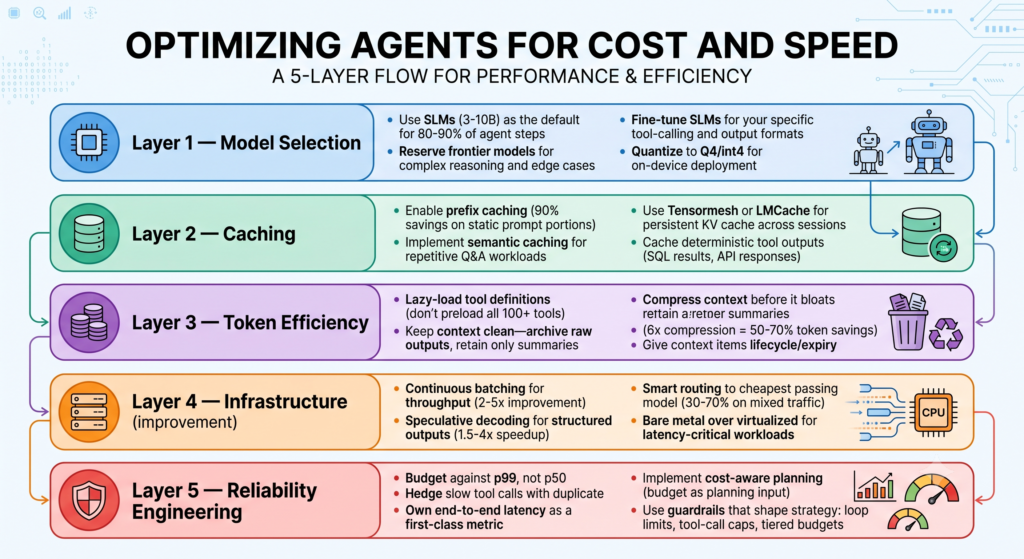
Expected Combined Savings

Teams implementing the full stack is expected to have:

60–90% cost reduction vs naive single-frontier-model deployment
5–37x speed improvements for agent step latency
10x reduction in cost variance through proper guardrails and modeling
Break-even on dedicated hardware in days to weeks at production volume

The key principle: treat inference cost as a variable line in gross margin, not a fixed infrastructure expense. Measure, attribute, and optimize continuously.

Summary

Agentic AI systems amplify every inefficiency in LLM inference through their multi-step, multi-call nature. This chapter presented a comprehensive optimization stack that addresses cost and latency at every layer—from model selection (SLMs as the default) through caching (KV prefix, semantic), token efficiency (lazy-loading, context hygiene), infrastructure (batching, routing, quantization), and reliability engineering (tail latency control, cost-aware guardrails). Teams that implement this full stack achieve 60–90% cost reductions and order-of-magnitude speed improvements, transforming inference from an unpredictable expense into a manageable, optimizable line item.